Lecture 16 - Machine Learning: Intro/Overview; Vectors and Distances
Announcements:
Goals:
- See a few different perspectives on "what is machine learning?"
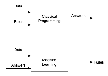
- CS/programmer's perspective
- DS/data wrangler's perspective
- Stats/mathematician's perspective
- Know the basic mathematical setup of most machine learning methods.
- Be able to give some example use cases where machine learning is the best, if not only practical, way to solve a computing problem.
- Know how to represent datapoints as vectors, and how to compute $L_p$ distances between them.
A data scientist's perspective:
A way to discover underlying structure in data that allows us to:
- Better understand the world that generated the data
- Predict values (columns, rows, subsets thereof) that are:
- missing (imputation), or
- haven't happened yet (prediction, time series forecasting, etc.)
A mathematical / probabilistic perspective:
Given a set of data $X$ and (possibly) labels $y$ (i.e., quantities to predict), model one or more of the following:
- $P(x)$
- $P(y \mid x)$
- $P(x, y)$.
Math Fact: If you know $P(x, y)$, you can compute $P(y \mid x)$ and $P(x)$:
$$P(y \mid x) = \frac{P(x, y)}{P(x)}$$ and $$P(x) = \sum_i P(x,y_i)$$
Machine Learning: When and Why?
- We don't know the underlying process that generated the data, but we have examples of its outputs
- Use cases: (so far) data-rich domains with problems we don't know how to solve any other way.
- High-profile examples are from complex domains:
- Speech recognition
- Image recognition / object detection
- Weather forecasting
- Natural Language Processing
- Self-driving cars (robotics)
- Drug design
Side note: Machine Learning vs. Artificial Intelligence
- AI is the study of making computer systems behave with "intelligence" (what does that mean?)
- ML is generally considered a subfield of AI
- ML has come the closest so far to exhibiting intelligent behavior
- Actively debated: is ML the way to "general" AI?
- In current usage, "AI" almost exclusively refers to ML-based methods
Supervised vs Unsupervised
Supervised Learning, by example:
- $X$ is a collection of $n$ homes with $d$ numbers about each one (square feet, # bedrooms, ...); $\mathbf{y}$ is the list of market values of each home.
Key property: a dataset $X$ with corresponding "ground truth" labels $\mathbf{y}$ is available, and we want be able to to predict a $y$ given a new $\mathbf{x}$.
Unsupervised Learning, by example:
- Same setup, but instead of predicting $y$ for a new $\mathbf{x}$, you want to know which of the $d$ variables most heavily influences home price.
Key property: you aren't given "the right answer" - you're looking to discover structure in the data.
import seaborn as sns
import numpy as np
Feature Extraction
The vast majority of machine learning methods assume each of your input datapoints is represented by a feature vector.
If it's not, it's usually your job to make it so - this is called feature extraction. mk Given a DataFrame, we can treat each row as the feature vector for the thing the row describes. Traditionally, we arrange our dataset in an $N \times D$ matrix, where each row corresponds to a datapoint and each column corresponds to a single feature (variable). This is the same layout as a pandas table.
If your input is an audio signal, a sentence of text, an image, or some other not-obviously-vector-like thing, there may be more work to do.
Given a dataframe like the penguins dataset, it's pretty easy to get to a ML-style training dataset X, y:
penguins = sns.load_dataset("penguins")
sns.relplot(data=penguins, x="flipper_length_mm", y="bill_length_mm")
X = penguins[["flipper_length_mm", "bill_length_mm"]].to_numpy()
X.shape
X[:10,:]
penguins["species"].value_counts()
y = penguins["species"].map({"Gentoo": 1, "Adelie": 2, "Chinstrap": 3}).to_numpy()
y.shape
y
Distance Metrics
So you have your datapoints represented as vectors. The big thing this enables is for us to compare two datapoints numerically - this is done by computing a disance (or inversely, similarity) between two datapoints.
$L^p$ Distances
A common family of distance metrics is the $L^p$ distance:
$$d_p(a, b) = \sqrt[p]{\sum_{i=1}^d |a_i - b_i|^p}$$
When $p = 2$, this is the Euclidean distance we're all used to, based on the Pythagorean theorem; in 2D, it reduces to: $$\sqrt{(b_x - a_x)^2 + (b_y - a_y^2)}$$
Different values of $p$ give different behavior:
- For smaller $p$, we care less about how different the per-dimension differences are from each other.
- For larger $p$, we care more about how different the per-dimension differences are from each other.
A few examples of the "unit circle" under different $L^p$ distances:
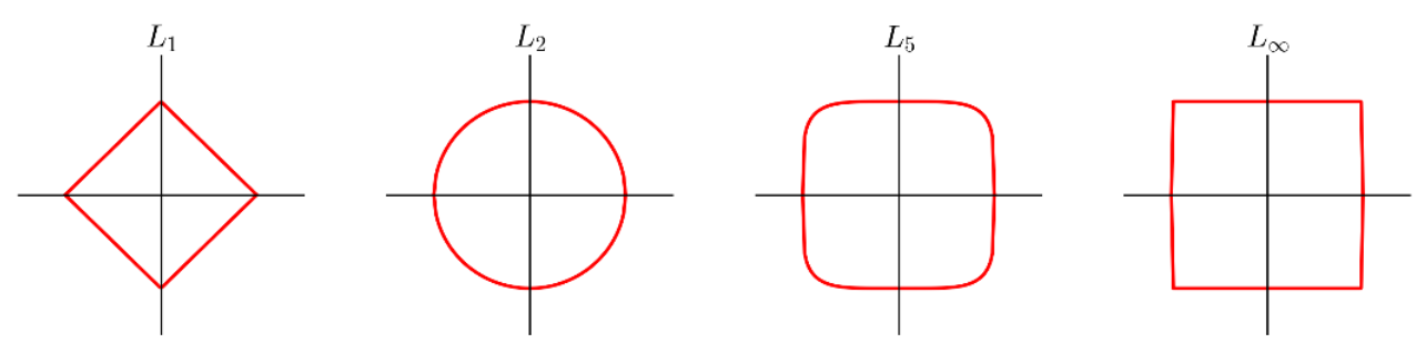
$L_1$ and $L_2$ are by far the most common choices here.
Exercise: rank the penguins by similarity to Penguin 0, based on an L2 distance between flipper + bill length vectors.
X[0]
penguins.iloc[0,:]
More Distance Metrics
Hamming Distance
For vectors of categorical values, Hamming distance is the number of dimensions in which two vectors differ: $$d(a, b) = \sum_i \mathbb{1}(a_i \ne b_i)$$ where $\mathbb{1}(\cdot)$ is an indicator function that has value 1 if its argument is true and 0 otherwise.
Cosine Similarity
A similarity (not distance) metric that considers only vector direction, not magnitude:
$$ sim(a, b) = \cos \theta = \frac{a^Tb}{\sqrt{(a^Ta)(b^Tb)}}$$