In [21]:
penguins = sns.load_dataset("penguins")
sns.relplot(data=penguins, x="flipper_length_mm", y="bill_length_mm")
Out[21]:
<seaborn.axisgrid.FacetGrid at 0x7facae30b4f0>

import pandas as pd
import seaborn as sns
import matplotlib.pyplot as plt
The vast majority of machine learning methods assume each of your input datapoints is represented by a feature vector.
If it's not, it's usually your job to make it so - this is called feature extraction.
Given a DataFrame, we can treat each row as the feature vector for the thing the row describes. Traditionally, we arrange our dataset in an $N \times D$ matrix, where each row corresponds to a datapoint and each column corresponds to a single feature (variable). This is the same layout as a pandas table.
If your input is an audio signal, a sentence of text, an image, or some other not-obviously-vector-like thing, there may be more work to do.
Given a dataframe like the penguins dataset, it's pretty easy to get to a ML-style training dataset X, y:
penguins = sns.load_dataset("penguins")
sns.relplot(data=penguins, x="flipper_length_mm", y="bill_length_mm")
<seaborn.axisgrid.FacetGrid at 0x7facae30b4f0>
X = penguins[["flipper_length_mm", "bill_length_mm"]].to_numpy()
X.shape
(344, 2)
X[:10,:]
array([[181. ,  39.1],
       [186. ,  39.5],
       [195. ,  40.3],
       [  nan,   nan],
       [193. ,  36.7],
       [190. ,  39.3],
       [181. ,  38.9],
       [195. ,  39.2],
       [193. ,  34.1],
       [190. ,  42. ]])
penguins["species"].value_counts()
Adelie       152
Gentoo       124
Chinstrap     68
Name: species, dtype: int64
y = penguins["species"].map({"Gentoo": 1, "Adelie": 2, "Chinstrap": 3}).to_numpy()
y.shape
(344,)
y
array([2, 2, 2, 2, 2, 2, 2, 2, 2, 2, 2, 2, 2, 2, 2, 2, 2, 2, 2, 2, 2, 2,
       2, 2, 2, 2, 2, 2, 2, 2, 2, 2, 2, 2, 2, 2, 2, 2, 2, 2, 2, 2, 2, 2,
       2, 2, 2, 2, 2, 2, 2, 2, 2, 2, 2, 2, 2, 2, 2, 2, 2, 2, 2, 2, 2, 2,
       2, 2, 2, 2, 2, 2, 2, 2, 2, 2, 2, 2, 2, 2, 2, 2, 2, 2, 2, 2, 2, 2,
       2, 2, 2, 2, 2, 2, 2, 2, 2, 2, 2, 2, 2, 2, 2, 2, 2, 2, 2, 2, 2, 2,
       2, 2, 2, 2, 2, 2, 2, 2, 2, 2, 2, 2, 2, 2, 2, 2, 2, 2, 2, 2, 2, 2,
       2, 2, 2, 2, 2, 2, 2, 2, 2, 2, 2, 2, 2, 2, 2, 2, 2, 2, 2, 2, 3, 3,
       3, 3, 3, 3, 3, 3, 3, 3, 3, 3, 3, 3, 3, 3, 3, 3, 3, 3, 3, 3, 3, 3,
       3, 3, 3, 3, 3, 3, 3, 3, 3, 3, 3, 3, 3, 3, 3, 3, 3, 3, 3, 3, 3, 3,
       3, 3, 3, 3, 3, 3, 3, 3, 3, 3, 3, 3, 3, 3, 3, 3, 3, 3, 3, 3, 3, 3,
       1, 1, 1, 1, 1, 1, 1, 1, 1, 1, 1, 1, 1, 1, 1, 1, 1, 1, 1, 1, 1, 1,
       1, 1, 1, 1, 1, 1, 1, 1, 1, 1, 1, 1, 1, 1, 1, 1, 1, 1, 1, 1, 1, 1,
       1, 1, 1, 1, 1, 1, 1, 1, 1, 1, 1, 1, 1, 1, 1, 1, 1, 1, 1, 1, 1, 1,
       1, 1, 1, 1, 1, 1, 1, 1, 1, 1, 1, 1, 1, 1, 1, 1, 1, 1, 1, 1, 1, 1,
       1, 1, 1, 1, 1, 1, 1, 1, 1, 1, 1, 1, 1, 1, 1, 1, 1, 1, 1, 1, 1, 1,
       1, 1, 1, 1, 1, 1, 1, 1, 1, 1, 1, 1, 1, 1])
Goal: discover structure without any ground-truth labels.
What might we mean by structure? A non-exhaustive list:
This is hard, and our intuition tends to fall apart. However, real high-dimensional data often lies on a lower-dimensional manifold.
What the heck does that mean?
If you sliced, rotated, projected, warped, etc. your space in just the right ways, you could represent the same information with fewer dimensions. The smallest possible number of dimensions possible to represent your data is called its intrinsic dimensionality.
Ways to get your $n$ feature vectors from $d$ dimensions to $d'$ dimensions (where $d' < d$).
Good for:
in all cases, these likely come at the expense of some accuracy.
Here are two common approches that are limited to linear notions of stretching, slicing, warping, etc:
Reduces dimensionality by finding $d'$ new features (each is a linear combination of the old features) that explain as much variance as possible.
Reduces dimensionality by multiplying $X_{n \times d}$ by a random matrix $P_{d \times d'}$, resulting in a reduced-dimensionality dataset $X'_{n \times d'}$.
Huh?
Somewhat surprisingly, this works pretty well.
Question: What's our metric for "works"?
Answer: It preserves pairwise distances between points.
A common family of distance metrics is the $L^p$ distance:
$$d_p(a, b) = \sqrt[p]{\sum_{i=1}^d |a_i - b_i|^p}$$When $p = 2$, this is the Euclidean distance we're all used to, based on the Pythagorean theorem; in 2D, it reduces to: $$\sqrt{(b_x - a_x)^2 + (b_y - a_y^2)}$$
Different values of $p$ give different behavior:
A few examples of the "unit circle" under different $L^p$ distances:
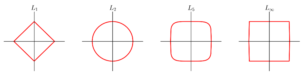
$L_1$ and $L_2$ are by far the most common choices here.
For vectors of categorical values, Hamming distance is the number of dimensions in which two vectors differ: $$d(a, b) = \sum_i \mathbb{1}(a_i \ne b_i)$$ where $\mathbb{1}(\cdot)$ is an indicator function that has value 1 if its argument is true and 0 otherwise.
A similarity (not distance) metric that considers only vector direction, not magnitude:
$$ sim(a, b) = \cos \theta = \frac{a^Tb}{\sqrt{(a^Ta)(b^Tb)}}$$It's worth noting that many distance metrics become less and less useful as $d$ gets larger. There are a few ways to think about this, but the simplest is just that more dimensions means more opportunities for points to be far apart.
Cosine similarity is often better in high dimensions this because it ignores magnitude.
An example of using PCA on a synthetic dataset:
# Authors: Gael Varoquaux
#          Jaques Grobler
#          Kevin Hughes
# Adapted by Scott Wehrwein for DATA 311
# License: BSD 3 clause
%matplotlib inline
import sklearn
import sklearn.decomposition

from mpl_toolkits.mplot3d import Axes3D
import numpy as np
import matplotlib.pyplot as plt
from scipy import stats


# #############################################################################
# Create the data

e = np.exp(1)
np.random.seed(4)


def pdf(x):
    return 0.5 * (stats.norm(scale=0.25 / e).pdf(x) + stats.norm(scale=4 / e).pdf(x))


y = np.random.normal(scale=0.5, size=(30000))
x = np.random.normal(scale=0.5, size=(30000))
z = np.random.normal(scale=0.1, size=len(x))

density = pdf(x) * pdf(y)
pdf_z = pdf(5 * z)

density *= pdf_z

a = x + y
b = 2 * y
c = a - b + z

norm = np.sqrt(a.var() + b.var())
a /= norm
b /= norm


# #############################################################################
# Do PCA and plot a figure showing the data and the plane spanned by the first 2
# PCs
def plot_figs(fig_num, elev, azim):
    Y = np.c_[a, b, c]

    pca = sklearn.decomposition.PCA(n_components=3)
    pca.fit(Y)
    V = pca.components_.T

    # from here on is just plotting stuff:
    fig = plt.figure(fig_num, figsize=(8, 5))
    plt.clf()
    ax = Axes3D(fig, rect=[0, 0, 0.95, 1], elev=elev, azim=azim)

    ax.scatter(a[::10], b[::10], c[::10], c=density[::10], marker="+", alpha=0.4)


    x_pca_axis, y_pca_axis, z_pca_axis = 3 * V
    x_pca_plane = np.r_[x_pca_axis[:2], -x_pca_axis[1::-1]]
    y_pca_plane = np.r_[y_pca_axis[:2], -y_pca_axis[1::-1]]
    z_pca_plane = np.r_[z_pca_axis[:2], -z_pca_axis[1::-1]]
    x_pca_plane.shape = (2, 2)
    y_pca_plane.shape = (2, 2)
    z_pca_plane.shape = (2, 2)
    ax.plot_surface(x_pca_plane, y_pca_plane, z_pca_plane)
    ax.w_xaxis.set_ticklabels([])
    ax.w_yaxis.set_ticklabels([])
    ax.w_zaxis.set_ticklabels([])

    ax.set_xlabel("x")
    ax.set_ylabel("y")
    ax.set_zlabel("z")
    print("Component Vectors (one per column):")
    print(pca.components_.T)
    print("Explained variance:")
    print(pca.explained_variance_)
plot_figs(1, 0, 0)
Component Vectors (one per column):
[[-0.33847725 -0.7109608   0.61641536]
 [-0.77400604 -0.1621726  -0.61205775]
 [ 0.53511475 -0.68427684 -0.49539622]]
Explained variance:
[1.0908032  0.41318925 0.00246436]

elev = 30
azim = 20
plot_figs(2, elev, azim)

plt.show()
Component Vectors (one per column):
[[-0.33847725 -0.7109608   0.61641536]
 [-0.77400604 -0.1621726  -0.61205775]
 [ 0.53511475 -0.68427684 -0.49539622]]
Explained variance:
[1.0908032  0.41318925 0.00246436]

Find clusters of points based on proximity, density, or other similar metrics.
Example algorithm: K means
Demo: https://www.naftaliharris.com/blog/visualizing-k-means-clustering/
penguins = sns.load_dataset("penguins")
sns.relplot(data=penguins, x="flipper_length_mm", y="bill_length_mm")
<seaborn.axisgrid.FacetGrid at 0x7faca7787cd0>
Xdf = penguins[["flipper_length_mm", "bill_length_mm"]].dropna()
X = Xdf.to_numpy()
X.shape
(342, 2)
from sklearn.cluster import KMeans

kmeans = KMeans(n_clusters=3)
kmeans.fit(X)

Xdf["cluster"] = kmeans.labels_

Xdf.info()
<class 'pandas.core.frame.DataFrame'>
Int64Index: 342 entries, 0 to 343
Data columns (total 3 columns):
 #   Column             Non-Null Count  Dtype
---  ------             --------------  -----
 0   flipper_length_mm  342 non-null    float64
 1   bill_length_mm     342 non-null    float64
 2   cluster            342 non-null    int32
dtypes: float64(2), int32(1)
memory usage: 9.4 KB
kmeans.cluster_centers_
array([[196.7311828 ,  45.95483871],
       [216.88372093,  47.56744186],
       [186.99166667,  38.4275    ]])
fig = plt.figure()
plt.subplot(1,2,1)
sns.scatterplot(data=Xdf, x="flipper_length_mm", y="bill_length_mm", hue="cluster")
plt.scatter(x=kmeans.cluster_centers_[:,0], y=kmeans.cluster_centers_[:,1], c="red", marker="x")
plt.subplot(1,2,2)
sns.scatterplot(data=penguins, x="flipper_length_mm", y="bill_length_mm", hue="species")
plt.show()

sns.relplot(data=penguins, x="flipper_length_mm", y="bill_length_mm", hue="species")