Lecture 16 - Machine Learning - Taxonomy, The In-Distribution Assumption

import pandas as pd
import seaborn as sns

df = pd.DataFrame({
  "Income": [0.49, 0.18, 0.31, 0.40, 0.24],
  "CrimeRate": [0.09, 0.45, 0.23, 0.19, 0.48]
})

Announcements:

• Lab 5: Please scrape the-numbers pages from the mirrored version hosted on my webpage.
  • Deadline extended to Sunday (2/19) night at 10pm
  • Future labs are unaffected: Lab 6 out Friday, due Thursday as usual.
• Quiz 4 - the multiple-answer numpy question: needs manual regrading, I will get to this Soon(TM).
• Data ethics 2 due tomorrow!

Quiz 5

• Question 1 still needs manual grading - Soon(TM)
• Scores quite good overall! FMQ:
  • soup.element and soup.find(element) both give you the first instance of element in the soup
  • soup.find_all returns a list (even if it's an empty one)

Goals:

• Understand the near-universal assumption of machine learning models: unseen data is drawn from the same distribution as the training dataset, and the implications of this assumption.

• Understand the meaning of and distinction between unsupervised learning and supervised learning.

• Understand the meaning of and distinction between discriminative and generative learning.

• Know how to define bias, variance and irreducible error

• Be able to identify the most common causes of the above types of error, and explain how they relate to generalization, risk, overfitting, underfitting.

Terminology Review

• Model Class
• Loss function
• Empirical Risk

Bonus:

• training set
• Inputs / features / independent variables
• Labels / targets / dependent variables

From last time: Ok, how do we do this?

Overview: three steps:

1. Decide on a model class
2. Decide on a formal definition of how well a model fits the training data.
3. Optimize (search for the best model in the model class) - aka train, or learn

sns.scatterplot(data=df,x="Income",y="CrimeRate")

<matplotlib.axes._subplots.AxesSubplot at 0x7f514df850a0>

Step 1: Decide on a model class

• There are a ton of options, since this looks vaguely linear, let's keep it simple:
  • Model class: linear functions; i.e., $h(x) = mx + b$
    • $x$ is the input
    • $m$ (slope) and $b$ (y-intercept) are the parameters of the model.
    • Equivalent terminology: $m$ and $b$ are weights, or $m$ is a weight and $b$ is a bias.

Step 2: Decide on a formal definition of how well a model fits the training data.

• Break this into two substeps:
  1. Define a loss function that indicates how poorly the model does on a single datapoint. Here, we choose to use squared error loss (lots of alternative options):
  $$ L(h(x),y) = (h(x)-y)^2$$
  • Loss functions are typically 0 when the prediction is correct
  • Loss functions grow as the prediction is more wrong
  • Squared error loss is popular because it is (relatively) easy to optimize
  2. Compute the *empirical risk* (i.e., average loss over the training set)
  $$ \hat{R}(h; {\cal X}) = \frac{1}{N} \sum_{i=1}^N L(h(x_{(i)}),y_{(i)})$$
  • $h$ is the model
  • ${\cal X}$ is the training set
  • $\sum$ is adding up losses for datapoints $1,2,\dots,N$
  • Note that ${\cal X}$ is fixed -- this is a function of $h$, which in our case, means it is a function of $m$ and $b$.

Step 3: Optimize

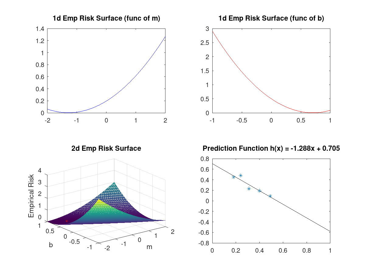
Training means solving the following optimization problem: $$ h^* = \arg\min_{h} \hat{R}(h; {\cal X})$$ Let's break this down:

• $h^*$ the optimal model (i.e., the line with the best $m$ and $b$)
• $\arg\min_h$ means to find and return the $h$ that gives the smallest value of the function being minimized
• $\hat{R}(h; {\cal X})$ the function being minimized

Solving this problem requires math we can't count on in this class, so let's jump to the solution: $$ h^*(x) \approx -1.29x + 0.71$$

Plot of solution

Taxonomic Considerations

Classification vs Regression

A way to describe a prediction task, depending on the value(s) being predicted:

• If outputs are real-valued (continuous): this is a regression task.

  • What is the sentiment (or polarity) of this sentence, on a scale from -1 to 1?
  • Given average per capita income, what is the crime rate of a city?

• If outputs are categorical (discrete): this is a classification task.

  • Does this image have a cat?
  • Which of a fixed set of 1000 objects does this image depict?

Supervised vs Unsupervised

Supervised Learning, by example:

• $X$ is a collection of $n$ homes with $d$ numbers about each one (square feet, # bedrooms, ...); $\mathbf{y}$ is the list of market values of each home.

Key property: a dataset $X$ with corresponding "ground truth" labels $\mathbf{y}$ is available, and we want be able to to predict a $y$ given a new $\mathbf{x}$.

Unsupervised Learning, by example:

• Same setup, but instead of predicting $y$ for a new $\mathbf{x}$, you want to know which of the $d$ variables most heavily influences home price.

Key property: you aren't given "the right answer" - you're looking to discover structure in the data.

Reminder: A mathematical / probabilistic perspective:

Given a set of data $X$ and (possibly) labels $y$ (i.e., quantities to predict), model either $P(y | x)$ or $P(x, y)$.

Recall: If you know $P(x, y)$, you can compute $P(y | x)$:

$$P(y | x) = \frac{P(x, y)}{P(x)}$$

and $$P(x) = \sum_i P(x,y_i)$$

Let's apply this probabilistic interpretation to our crime rate prediction task:

sns.scatterplot(data=df,x="Income",y="CrimeRate")

<matplotlib.axes._subplots.AxesSubplot at 0x7f514db306d0>

Discriminative vs Generative

For the moment, let's focus on supervised classification for the moment. In this case, $\mathbf{x}$ is a vector and $y$ is a discrete label indicating one of a set of categories or classes.

Discriminative models try to estimate $P(y | \mathbf{x})$. If you know this, then pick the most likely label, i.e., the $y$ that maximizes $P(y | \mathbf{x})$, and that's your predicted label for $\mathbf{x}$.

• Example: image classification

Generative models try to estimate $P(\mathbf{x})$ (if there are no labels $y$), or $P(x, y)$ if labels exist.

• Example: image generation

Note: it's easy to conclude that classification and discriminative are the same thing; they're not! Classifiers are often discriminative, but not always. How does that work?

Consider two schemes for classifying penguin species given their bill length and depth.

Exercise: Which of these is generative and which is discriminative?

1. Draw lines through the space and classify based on which area the penguin is in:
2. Fit 2D Gaussian distributions to the three species, and classify based on which Gaussian says a point is most probable:

Exercises:

1. Automatically detecting outlier images - like lab 4, except fully automatic.

   • Classification, regression, or neither?
   • Supervised or unsupervised?

2. Using linear regression (i.e., a best-fit line) to predict home value based on square feet given a set of actual home data from Zillow.

   • Classification, regression, or neither?
   • Supervised or unsupervised?

3. Finding "communities" of people who frequently interact with each other on a social network given a dataset of information about their social interactions on the network.

   • Classification, regression, or neither?
   • Supervised or unsupervised?

Assumptions

Data distribution

Generally: unseen data is drawn from the same distrubtion as your dataset.

Consequence: We don't assume correlation is causation, but we do assume that observed correlations will hold in unseen data.

Specific models: many more!

For example, linear regression assumes:

• Columns are linearly independent (i.e., one column can't be directly computed from another
• Data is homoscedastic, i.e., the following won't happen:

Big Idea: Generalization

Generalization is the ability of a model to perform well on unseen data (i.e., data that was not in the training set).

sns.scatterplot(data=df,x="Income",y="CrimeRate")

We limited our model class to linear functions. What other choices might we make?

• Quadratic?
• Piecewise linear?
• Higher-order polynomial?

What effect does this choice have on the optimal value of $\hat{R}(h; \mathcal{X})$?

What effect does this choice have on the model's ability to generalize to unseen data?

Empirical Risk vs True Risk

What we truly care about is a quantity known as (true) risk: $R(h; {\cal X})$.

• Risk is the expected loss "in the wild"
• Depends on a probability distribution that we don't know. Depends on $P(x,y)$ -- probability of each input-output pair.
  • If we knew $P$, there's nothing left to "learn."

There are three contributors to risk:

1. Bias (not the same bias as the $b$ in our linear model)
2. Variance
3. Irrereducible error

To understand bias and variance, we need to consider hypothetical:

• There is some underlying distribution/source generating input-output pairs
  • The probabily of a pair is denoted $P(x,y)$
  • The probability of the output given the input is denoted $P(y|x)$
  • Why a distribution? Because the same input (x) can have different ouputs (y).
• for i in 1..K
  • Get a random training set with $N$ points sampled from $P$
  • Train a model on that training set, call that $h_i(x)$.
• Define $\bar{h}(x) = \frac{1}{N} \sum_{i=1}^K h_i(x)$

Bias

• The bias of the training process is how far $\bar{h}(x)$ is from the mean of $P(y|x)$.
• High bias implies something is keeping you from capturing true behavior of the source.
• Most common cause of bias? The model class is too restrictive aka too simple aka not powerful enough aka not expressive enough.
  • E.g., if the true relationship is quadratic, using linear functions will have high bias.
• Training processes with high bias are prone to underfitting.
  • Underfitting is when you fail to capture important phenomena in the input-output relationship, leading to higher risk.

Variance

• The variance of a training process is the variance of the individual models $h_i(x)$; that is, how spread they are around $\bar{h}(x)$.
• This is a problem, because we only have one $h_i$, not $\bar{h}(x)$, so our model might be way off even if the average is good.
• Most common causes of variance?
  • Too powerful/expressive of a model, which is capable of overfitting the the training. Overfitting means memorizing or being overly influenced by noise in the training set.
  • Small training set sizes ($N$).
  • Higher irreducible error (noisier training set).

Irreducible Error

• Even if you have a zero bias, zero variance training process, you then predict the mean $P(y|x)$, which is almost never right.
  • Because the truth is non-deterministic.
  • This error that remains is the irreducible error.
• Source of irreducible error?
  • Not having enough, or enough relevant features in $x$.
• Note: this error is only irreducible for a given feature set (the information in $x$). If you change the problem to include more features, you can reduce irreducible error.