CSCI 497P/597P: Computer Vision, Winter 2019
Project 2: Feature Detection and Matching
Brief
- Released: Tuesday, January 22, 2019
- Code Due: Wednesday, January 30, 2019 (by 9:59 PM) (submission via Github)
- Report Due: Friday, February 1, 2019 (by 9:59 PM) (submission via Canvas)
- Teams: The code for this assignment must be done in groups of 2 students. Both members of a group must be in the same section of the course (497P or 597P). The report must be created indivudally.
Synopsis
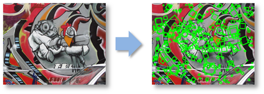
The goal of feature detection and matching is to identify a pairing between a point in one image and a corresponding point in another image. These correspondences can then be used to stitch multiple images together into a panorama (Project 3), or in various other computer vision applications (examples given in lecture).
In this project, you will write code to detect discriminating features (which are reasonably invariant to translation, rotation, and illumination) in an image and find the best matching features in another image.
To help you visualize the results and debug your program, we provide a user interface that displays detected features and best matches in another image. We also provide an example ORB feature detector, a popular technique in the vision community, for comparison. ORB is intended as a replacement for SIFT: it builds on the FAST keypoint detector and the BRIEF feature descriptor.
Description
The project has three parts: feature detection, feature description, and feature matching.
1. Feature detection
In this step, you will identify points of interest in the image using the Harris corner detection method. The steps are as follows (see the lecture slides and textbook for more details). For each point in the image, consider a window of pixels around that point. Compute the Harris matrix H for (the window around) that point, defined as
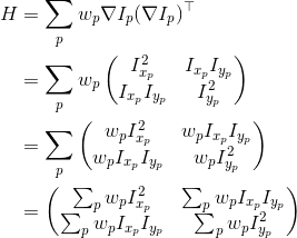
where the summation is over all pixels p in the
window.  is the x derivative of the image at point p, the notation is similar for the y derivative. You should use the 3x3 Sobel operator to compute the x, y derivatives (extrapolate pixels outside the image with reflection). The weights
  should
be circularly symmetric (for rotation invariance) - use a 5x5 Gaussian mask with 0.5 sigma (or you may set Gaussian mask values more than 4 sigma from the mean to zero. This is within tolerance.). Use reflection for gradient values outside of the image range. Note that H is a 2x2 matrix.
should
be circularly symmetric (for rotation invariance) - use a 5x5 Gaussian mask with 0.5 sigma (or you may set Gaussian mask values more than 4 sigma from the mean to zero. This is within tolerance.). Use reflection for gradient values outside of the image range. Note that H is a 2x2 matrix.
Then use H to compute the corner strength function, c(H), at every pixel.

We will also need the orientation in degrees at every pixel. Compute the approximate orientation as the angle of the gradient. The zero angle points to the right and positive angles are counter-clockwise. Note: do not compute the orientation using eigen analysis of the structure tensor.
We will select the strongest keypoints (according to c(H)) which are local maxima in a 7x7 neighborhood.
2. Feature description
Now that you have identified points of interest, the next step is to come up with a descriptor for the feature centered at each interest point. This descriptor will be the representation you use to compare features in different images to see if they match.
You will implement two descriptors for this project. For starters, you will implement a simple descriptor which is the pixel intensity values in the 5x5 neighborhood. This should be easy to implement and should work well when the images you are comparing are related by a simple translation.
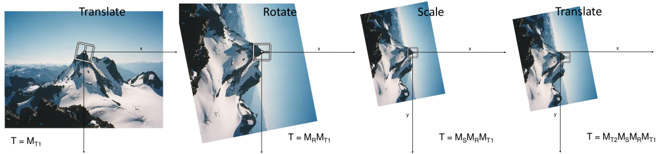
Second, you will implement a simplified version of the MOPS descriptor. You will compute an 8x8 oriented patch sub-sampled from a 40x40 pixel region around the feature. You have to come up with a transformation matrix which transforms the 40x40 rotated window around the feature to an 8x8 patch rotated so that its keypoint orientation points to the right. You should also normalize the patch to have zero mean and unit standard deviation. If the standard deviation is very close to zero (less than 10-5 in magnitude) then you should just return an all-zeros vector to avoid a divide by zero error.
You will use cv2.warpAffine to perform the transformation.
warpAffine takes a 2x3 forward warping affine matrix, which is
multiplied from the left with the input coordinates given as a column vector.
The easiest way to generate the 2x3 matrix is by combining a sequence of
translation (T1), rotation (R), scaling (S) and translation (T2) matrices.
Recall that a sequence of linear transformations left-multiplied by a vector
are applied applied right-to-left; this means that if the transformation
matrix is the matrix product T2 S R T1, then you perform the translation T1,
followed by the rotation R, then scale S, then another translation T2. The
figures below illustrate the sequence. You are provided with some utility
methods (more details below) in transformations.py that may help
you in constructing your transformation matrix.
3. Feature matching
Now that you have detected and described your features, the next step is to write code to match them (i.e., given a feature in one image, find the best matching feature in another image).
The simplest approach is the following: compare two features and calculate a scalar distance between them. The best match is the feature with the smallest distance. You will implement two distance functions:
- Sum of squared differences (SSD): This is the squared Euclidean distance between the two feature vectors.
- The ratio test: Find the closest and second closest features by SSD distance. The ratio test distance is ratio between the two, i.e., the SSD between the feature and its closest match divided by the SSD between the feature and its second closest match.
Testing and Visualization
Testing
You can test your TODO code by running "python tests.py". This will load a small image, run your code and compare against the correct outputs. This will let you test your code incrementally without needing all the TODO blocks to be complete.We have implemented tests for TODO's 1-6. You should design your own tests for TODO 7 and 8. Lastly, be aware that the supplied tests are very simple - they are meant as an aid to help you get started. Passing the supplied test cases does not mean the graded test cases will be passed.
Visualization
Now you are ready to go! Using the UI and skeleton code that we provide, you can load in a set of images, view the detected features, and visualize the feature matches that your algorithm computes. Watch this video to see the UI in action.
By running featuresUI.py, you will see a UI where you have the following choices:
- Keypoint Detection
You can load an image and compute the points of interest with their orientation. - Feature Matching
Here you can load two images and view the computed best matches using the specified algorithms. - Benchmark
After specifying the path for the directory containing the dataset, the program will run the specified algorithms on all images and compute ROC curves for each image.
The UI is a tool to help you visualize the keypoint detections and feature matching results. Keep in mind that your code will be primarily evaluated numerically, not visually.
Benchmarking
We provide a set of benchmark images to be used to test the performance of your algorithm as a function of different types of controlled variation (i.e., rotation, scale, illumination, perspective, blurring). For each of these images, we know the correct transformation and can therefore measure the accuracy of each of your feature matches. This is done using a routine that we supply in the skeleton code.
You should also go out and take some photos of your own to see how well your approach works on more interesting data sets. For example, you could take images of a few different objects (e.g., books, offices, buildings, trees, etc.) and see how well it works.
Getting Started
Skeleton. Find the Github Classroom invitation link in
the Project 2 assignment on Canvas. You will be writing code in
features.py. The user interface is given in
featuresUI.py - run this file with Python to start up the user
interface. Sample images and benchmarks are provided in the
resources subdirectory. Please keep track of the approximate
number of hours you spend on this assignment, as you will be asked to report
this in your writeup a file called hours.txt when you submit.
Software : The lab machines should have all the necessary software to run the code for this project. The dependencies for this project should be the same as the ones listed in Project 1 - please see the Project 1 writeup for details. If you encounter issues (especially if you find that there are additional dependencies missing), please post on Piazza so the writeup can be updated accordingly.
To Do
We have given you a number of classes and methods.
You are responsible for reading the code documentation and understanding the role of each class
and function.
The code you need to write will be for your feature detection methods,
your feature descriptor methods and your
feature matching methods. All your required edits will be in features.py.
The feature computation and matching methods are called from the UI functions in
featuresUI.py. Feel free to extend the functionality of the UI code but remember
that only the code in features.py will be graded.
597P students have one additional task (#4 below).
Details
-
The function
detectKeypointsinHarrisKeypointDetectoris one of the main ones you will complete, along with the helper functionscomputeHarrisValues(computes Harris scores and orientation for each pixel in the image) andcomputeLocalMaxima(computes a Boolean array which tells for each pixel if it is equal to the local maximum). These implement Harris corner detection. You may find the following functions helpful:scipy.ndimage.sobel: Filters the input image with Sobel filter.scipy.ndimage.gaussian_filter: Filters the input image with a Gaussian filter.scipy.ndimage.filters.maximum_filter: Filters the input image with a maximum filter.scipy.ndimage.filters.convolve: Filters the input image with the selected filter.
-
You will need to implement two feature
descriptors in
SimpleFeatureDescriptorandMOPSFeaturesDescriptorclasses. ThedescribeFeaturesfunction of these classes take the location and orientation information already stored in a set of key points (e.g., Harris corners), and compute descriptors for these key points, then store these descriptors in a numpy array which has the same number of rows as the computed key points and columns as the dimension of the feature (e.g., 25 for the 5x5 simple feature descriptor).For the MOPS implementation, you should create a matrix which transforms the 40x40 patch centered at the key point to a canonical orientation and scales it down by 5, as described in the lecture slides. You may find the functions in
transformations.pyhelpful, which implement 3D affine transformations (you will need to convert them to 2D manually). Reading the opencv documentation forcv2.warpAffineis recommended. -
Finally, you will implement a function for matching features. You will
implement the
matchFeaturesfunction ofSSDFeatureMatcherandRatioFeatureMatcher. These functions return a list ofcv2.DMatchobjects. These are simply struct-like objects with three fields:queryIdxtrainIdxdistance
queryIdxattribute to the index of the feature in the first image, the trainIdx attribute to the index of the feature in the second image and the distance attribute to the distance between the two features as defined by the particular distance metric (e.g., SSD or ratio). You may find scipy.spatial.distance.cdist and numpy.argmin helpful when implementing these functions. -
For 597P students only: Once you have completed all of the above tasks, make a copy of your
features.pyand save it asfeatures_scale_invariant.py, being sure to add it to your git repository. In this file, you will improve your implementation by making the descriptor scale-invariant. This means you will need to change the way features are detected, described, or both. How you do it is your design choice, but it should be well motivated. You may refer to the original MOPS paper to see how the authors accomplished scale invariance. You may choose to implement that, something else, or invent your own approach. You will describe your implementation and how it works in your writeup. In our codebase, the simplest approach is probably something like the following:- In
detectKeypoints, compute features on each layer of a Gaussian pyramid. - For each keypoint detected, fill in the
octavefield to indicate which level of the pyramid it was detected in. - In
describeFeatures, use theoctavevalue of the keypoint to modify the feature transformation matrix so that it extracts a patch from the original image that's equivalent to a 40x40 patch in the given level of the Gaussian pyramid. Alternatively, you could compute the Gaussian pyramid and use octave to decide which pyramid level to extract the descriptor from. You may want to look up OpenCV's built-in functions for creating Gaussian pyramids.
- In
-
For all students: Create a short report (details below), which includes benchmarking results in terms of ROC curves and AUC on the
Yosemitedataset provided in theresourcesdirectory. You can obtain ROC curves by running featuresUI.py, switching to the "Benchmark" tab, pressing "Run Benchmark", selecting the directory "resources/yosemite" and waiting a short while. Then the AUC will be shown on the bottom of the screen and you may save the ROC curve by pressing "Screenshot". You will also need to include one harris image. This is saved asharris.png, every time the harris keypoints are computed.
Coding Rules
You may use NumPy, SciPy and OpenCV2 functions to implement mathematical, filtering and transformation operations. Do not use functions which implement keypoint detection or feature matching.
When using the Sobel operator or gaussian filter, you should use the 'reflect' mode, which gives a zero gradient at the edges.
Here is a list of potentially useful functions (you are not required to use them):
scipy.ndimage.sobelscipy.ndimage.gaussian_filterscipy.ndimage.filters.convolvescipy.ndimage.filters.maximum_filterscipy.spatial.distance.cdistcv2.warpAffinenp.max, np.min, np.std, np.mean, np.argmin, np.argpartitionnp.degrees, np.radians, np.arctan2transformations.get_rot_mx(intransformations.py)transformations.get_trans_mxtransformations.get_scale_mx
Submission
Code:
All Students: Push your finished code to Github. Create a file
called hours.txt in the repository's root directory that includes a single
lone integer estimate of the number of hours Include an estimate of the
number of hours you worked in a file called hours.txt in the repository's
root directory.
597P Students: Make sure your features_scale_invariant.py and readme_scale_invariant.txt are tracked in your repo and pushed to Github.
If you attempted the extra credit (see below) make sure extracredit.py and extracredit_readme.txt are tracked in your repo and pushed to Github. If you did not attempt the extra credit then you do not need to submit extracredit.py or extracredit_readme.txt (please do not include empty extra credit files).
Report:
Create a report in form of a pdf document or a small website describing your work and submit it to Canvas. If you submit a webpage, you should submit it as a zip file containing an index.html file along with any embedded files e.g. images. PDF reports should be submitted as report.pdf.
Your report should contain the following deliverables:
- At the top, give an estimate of the number of hours you spent working on this assignment. Count only the time you worked with or without your partner - do not count any time your partner spent working on it without you.
- Run the benchmark in featuresUI.py on the Yosemite dataset for the four possible configurations involving Simple or MOPS descriptors with SSD or Ratio distance. Include the resulting ROC curves, report AUC and comment which method is the best.
- Include the harris image on yosemite/yosemite1.jpg. Comment on what type of image regions are highlighted. Are there any image regions that should have been highlighted but aren't?
- Take a pair of your own images and visually show feature matching performance of MOPS + Ratio distance, by including a screenshot from featuresUI.py feature matching tab.
- (For 597P students) Describe how you made your descriptor scale invariant and justify your approach. Include ROC curves comparing your single-scale performance vs multi-scale performance on at least one of the benchmarks in the resources directory.
- (If you did extra credit) Include the ROC curve and report AUC from Yosemite dataset with your custom algorithm using ratio distance. Describe your changes to the algorithm and why they improve performance.
Extra Credit
We will give extra credit for solutions (feature detection and descriptors) that improve mean AUC for the ratio test by at least 15%. A 15% improvement is interpreted as a 15% reduction in (1 - AUC). i.e. the area above the curve. Here is one suggestion (and you are encouraged to come up with your own ideas as well!)
 Implement adaptive
non-maximum suppression (MOPS paper)
Implement adaptive
non-maximum suppression (MOPS paper)
If you attempt the extra credit then you must submit two solutions to CMS. The first solution will be graded by the project rubric so it must implement the algorithm described in this document. Extra credit solutions should include a readme that describes your changes to the algorithm and the thresholds for each benchmark image. The submitted code will be checked against this description. Extra credit submissions which do not improve mean AUC by at least 15% will not be graded. You can measure your mean AUC by running the UI benchmark on the 5 datasets (bikes, graf, leuven, wall, yosemite). We will specifically check performance on the yosemite dataset.
The extra credit will be given based on the merit of your improvement and its justification. Simple hyperparameter changes will receive less extra credit than meaningful improvements to the algorithm.
It is important that you solve the main assignment first before attempting the extra credit. The main assignment will be worth much more points than the extra credit.
Rubric
This project is worth a total of 50 points for 497P, and 60 points for 597P. Points are earned for correctness and efficiency, while deductions are possible for issues with clarity, coding style, or submission mechanics.
| Correctness (30 points) | |
| 30 points | Correctness as determined by automated tests. Some tests have large tolerances, so approximately correct solutions may receive partial credit. |
| Efficiency (10 points) | |
| 3 points | Corner detection is done with filtering routines |
| 3 points | Descriptor is computed with a single call to cv2.warpAffine |
| 4 points | Tests run within order of magnitude of the runtime the solution code, which contains no special optimizations. |
| Writeup (10 points) | |
| 4 points | ROC curves and AUC scores are reported for all four combinations of descriptor and distance metric. |
| 3 points | harris.png for yosemite/yosemite1.jpg and commentary |
| 2 points | Feature matching example on your own images |
| 1 point | Approximate number of hours you spent on the assignment is listed at the top of the writeup. |
| 597P Only (10 points) | |
| 5 points | Multiscale feature implementation |
| 5 points | Writeup - description of your multi-scale approach and ROC curves for at least one dataset. |
Clarity Deductions for poor coding style may be made. Please see the syllabus for general coding guidelines. Up to two points may be deducted for each of the following:
- Methods should be written as concisely and clearly as possible
- Methods should not be too long - use helper methods to break code into sensible subroutines
- Code should not be cryptic and terse - explain nontrivial blocks with comments
- Methods you introduce should be accompanied by a precise specification
- Variable and function names should be informative but not overly verbose
Submission Mechanics Up to 10 points may be deducted for problems with submission mechanics that require manual handling: for example, problems with your git repository, code that fails to run with the automated test suite, failure to notify me of your late submission, etc.
Acknowledgements
Many thanks are due to those who developed and refined prior versions of this assignment, including Steve Seitz, Kavita Bala, Noah Snavely, and many underappreciated TAs.