Lecture 2¶

Announcements¶

• Thanks for filling out the survey - office hours will be announced soon.
• Reminder that solutions for P01 and P02 are due Sunday night. Please typeset your answers.

Goals¶

• Know what is meant by image noise.
• Know how to filter (v) an image by cross-correlating it with a given filter (n)/kernel/weights
• Know how to handle image borders when filtering:
  • output sizes: full / same / valid
  • out-of-bounds values: zeros, reflection, replication

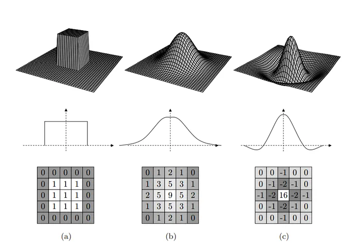
• Get a feel for some of the image processing operations that can and can't be accomplished using linear filtering.

  • Blur, sharpen, shift

• Know the properties of the convolution and cross-correlation, and some of their implications:

  • linearity, associativity, commutativity
  • separable filters and other compound operations

Lesson Plan¶

Syllabus questions

Revisiting image formation: image noise

Noise as motivation for neighborhood operations

Live code: mean filter

Edge handling choices:

• full, same, valid output size
• zero, reflect, repeat

Write down the discrete math definition; aside: write down the continuous definition

Live code: generalize to cross-correlation with filter weights

Mess with the filter weights:

• Horizontal blur
• Emboss

Exercise: compute a small cross-correlation result

Break

More filter weights:

• Left shift

Convolution vs cross-correlation

Properties - shift invariance; linearity; commutativity; associativity

Filter composition using associativity

Tricks using these properties:

• separable filters
• Blurring sequentially
• Sharpening

Image Formation Revisited¶

How do we record light intensity inside a camera?

• Film
• Digital sensors

Let's make beans a little noisy.

Brainstorm¶

If each pixel measurement is corrupted, how can we improve our guess at what the "ideal" image should have been?

Idea: mean filter

Live-pseudocode:

def mean_filter(img, filter_size):
    """ Apply a square spatial mean filter with side length filter_size
    to a grayscale img. Preconditions:
      - img is a grayscale (2d) float image
      - filter_size is odd """
    H, W = img.shape
    hw = filter_size // 2
    for i in range(H):
        for j in range(W):
            total = 0.0
            for ioff in range(-hw, hw+1):
                for joff in range(-hw, hw+1):
                    total += img[i + ioff, j + joff]
            out[i,j] = total / filter_size**2

Design Decisions - edge handling¶

(whiteboard)

Edge handling:

Output size:

• valid (only output where the whole filter overlaps the image)
• same (output same size as input)
• full (output everywhere the filter overlaps the image even a little bit)

For anything but valid, how do you handle when the filter hangs over the void?

• Zero padding
• Repeat (replicate) padding
• Reflect padding

Is a mean filter the best we can do?¶

Another example

See the lattice-like artifacts? Ick. Why is this happening?

Alternatives?

• Here's one:

TODO: implement filtering.filter

How would we calculate a Gaussian kernel ourselves?¶

where:

• $x, y$ are the spatial dimensions of the filter with (0,0) in the center of the kernel
• $\sigma$ is the standard deviation of the Gaussian, (determines how wide and flat vs tall and pointy it is)

Practicalities when calculating this in real life:

• You generally have to choose both a kernel size and a $\sigma$.
  • For a given kernel size, you can choose sigma so it fits $\pm$ 3 standard deviations, $\sigma = (k-1)/6$
  • Or for a given sigma, the kernel size that fits $\pm$ 3 standard deviations is $k = 2*\mathrm{ceil}(3*\sigma)+1$
• Not all the mass under the Gaussian fits in a finite kernel, so we usually renormalize the kernel so the weights sum to 1.

HW Problems 1 - 4¶

(1) $f \otimes w$ indicates the cross-correlation of image $f$ with filter $w$. Compute the following cross-correlation using same output size and zero padding. $$ \begin{bmatrix} 0 & 1 & 0\\ 0 & 1 & 0\\ 0 & 1 & 0 \end{bmatrix} \otimes \begin{bmatrix} 1 & 2 & 1\\ 2 & 4 & 2\\ 1 & 2 & 1 \end{bmatrix} $$

(2) Perform the same convolution as above, but use repeat padding.

(3) Perform the same convolution as above, but use valid output size.

(4) Describe in words the result of applying the following filter using cross-correlation. If you aren't sure, try applying it to the image above to gain intuition.

What else could we do with this?¶

Let's mess with filter weights to do weird stuff.

Break¶

Math definitions¶

Discrete cross-correlation:

Note that $g$ is defined with (0, 0) at the center.

Turns out there's a continuous version of this too! Sums become integrals:

Why $\infty$? Assume zero outside the boundaries.

Properties of Cross-Correlation¶

Convolution vs cross-correlation

Properties

• Linearity: if $a$ is a scalar, $f$ is an image, and $g$, $h$ are filters, then: $$\begin{align*} a(f \otimes g) = f \otimes ag = af \otimes g \\ (f \otimes g) + (f \otimes h) = f \otimes (g + h) \end{align*}$$
• Associativity $$ f \otimes (g \otimes h) = (f \otimes g) \otimes h $$
• Commutativity? $$ f \otimes g \overset{?}{=} g \otimes f $$ Check: $$ \begin{bmatrix} 0 & 0 & 0\\ 0 & 1 & 0\\ 0 & 0 & 0 \end{bmatrix} \otimes \begin{bmatrix} 1 & 2 & 3\\ 4 & 5 & 6\\ 7 & 8 & 9 \end{bmatrix} \overset{?}{=} \begin{bmatrix} 1 & 2 & 3\\ 4 & 5 & 6\\ 7 & 8 & 9 \end{bmatrix} \otimes \begin{bmatrix} 0 & 0 & 0\\ 0 & 1 & 0\\ 0 & 0 & 0 \end{bmatrix} $$

Aside: The filter above (with just a 1 in the middle) is called the identity filter.

Convolution¶

A small modification to cross-correlation yields Convolution:

Cross-correlation ($\otimes$): $$ (f \otimes g)(x, y) = \sum_{j=-\ell}^\ell \sum_{k=-\ell}^\ell f(x+j, y+k) * g(j, k) $$ Convolution ($*$): $$ (f * g)(x, y) = \sum_{j=-\ell}^\ell \sum_{k=-\ell}^\ell f(x-j, y-k) * g(j, k) $$

This effectively flips the filter horizontally and vertically before applying it, and gains us commutativity.

Okay, what can we do with these properties?¶

We can blur, but can we sharpen?¶

Key question: what did blurring remove?

$I - blur(I)$

What if we add back what's lost?

(whiteboard - equations here for posterity) \begin{align*} I' &= I + (I - (I * G))\\ &= (I + I) - (I * G))\\ &= (I * D) - (I * G)\\ &= I * (D - G)\\ \end{align*}

Visual intuition:

Efficiency trick: separable filters¶

Homework Problems 9-10:

1. Compute a 3x3 filter by convolving the following $1 \times 3$ filter with its transpose using full output size and zero padding: $$ \begin{bmatrix} 1 & 2 & 1\\ \end{bmatrix} $$

2. Suppose you have an image $F$ and you want to apply a $3 \times 3$ filter $H$ like the one above that can be written as $H = G * G^T$, where $G$ is $1 \times 3$. Which of the following will be more efficient?

   • $F * (G * G^T)$
   • $(F * G) * G^T$

What can't we do with convolution?¶

Homework Problem 11:

(11) For each of the following, decide whether it's possible to design a convolution filter that performs the given operation.

• Max filter: the output pixel is the maximum value among the pixels in the input window

• Threshold: the output pixel is

  • 255 if the input pixel is > 127
  • 0 otherwise
• $y$ partial derivative: the output is a finite-differences approximation of the input image's vertical derivative $\frac{\partial}{\partial y} f(x, y)$.