There is an equivalent lemma that can be used to show that a language is not context-free. The intuition is similar, except instead of “looping” journies through a state machine, we observe that subtrees of the parse tree must be repeated. We won’t cover this in much detail, but here’s the lemma:
Lemma (The Pumping Lemma for Context-Free Languages): Let \(L\) be a context-free language. Then there exists an integer \(p \ge 1\), called the pumping length, such that every string \(s\) in \(L\) with \(|s| \ge p\) can be written as \(s = uvxyz\), where
This can be used to prove, for example, that \(A = \{a^nb^nc^n : n \ge 0\}\) is not context-free.
Proof Sketch: Consider the string \(a^p b^p c^p\), and looks quite similar to the \(a^nb^n\) regular proof, except that we have to address three cases for the location of \(vxy\). Since \(u\) and/or \(w\) could be empty, we consider three cases:
Thus there’s no way to break \(s\) into \(uvxyz\) that satisfies the CF pumping lemma criteria, so the language cannot be context-free.
Having studied finite automata and pushdown automata, we now turn to our next more powerful machine, which turns out to be the most powerful one in the Chomsky Hierarchy. This is the famous Turing Machine, which turns out to be powerful enough to model any computer we know how to build (any classical computer, anyway - quantum computing is a different thing).
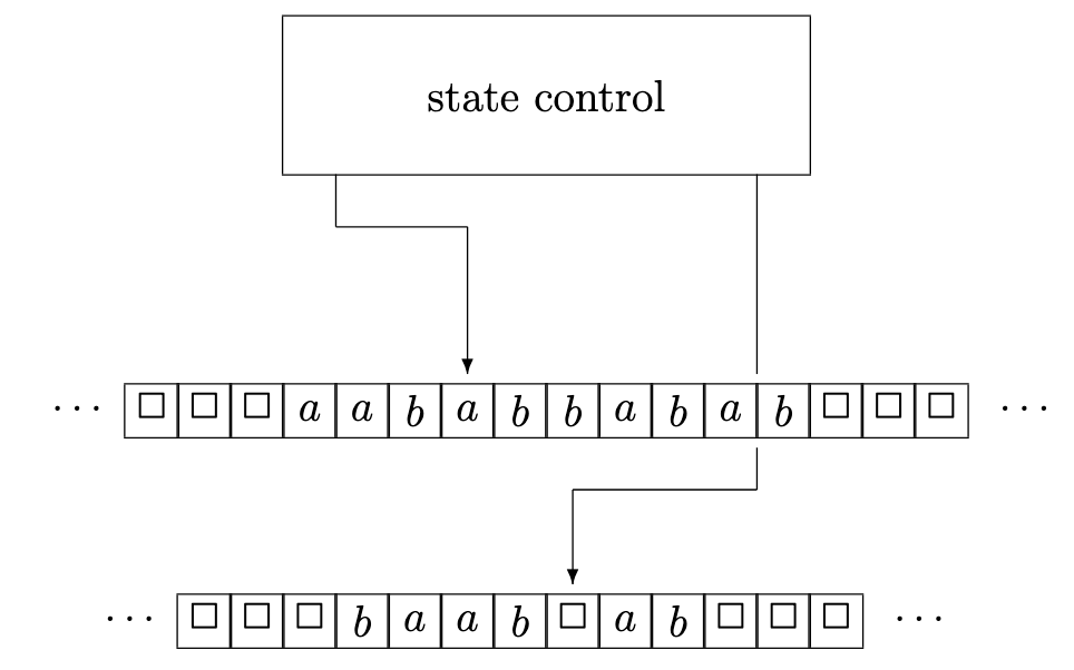
Informally, a Turing machine is similar to a PDA except that instead of a separate (read-only) input tape and mutable stack, we now have 1 or more tapes that can be read and/or written. Each tape head is now free to move left or right along each tape, and a computation step can involve overwriting the contents of a tape cell. Here’s a sketch from the textbook:
Formally, a deterministic \(k\)-tape turing machine is a 7-tuple \(M = (\Sigma, \Gamma, Q, \delta, q, q_{accept}, q_{reject})\), where
\(\Sigma\) is an alphabet not containing the blank symbol \(\square\)
\(\Gamma\) is a tape alphabet where \(\Sigma \subseteq \Gamma\) and \(\square \in \Gamma\)
\(Q\) is a finite set of states
\(q \in Q\) is the start state
\(q_{accept} \in Q\) is the accept
\(q_{reject} \in Q\) is the reject state
\(\delta\) is the transition function, which is a function \[ \delta : Q \times \Gamma^k \rightarrow Q \times \Gamma^k \times \{L, R, N\}^k. \]
Input: the transition function \(\delta\) takes as input:
Output: the output of the transition function is:
Initialization: The input string is stored on the first tape, with the first tape head on the leftmost symbol. The remainder of this and all other tapes is filled with the blank symbol \(\square\). The machine is in state \(q\), the start state.
Termination: The machine terminates immediately upon entering either the accept state \(q_{accept}\) or the reject state \(q_{reject}\).
Acceptance: The machine accepts a string if the computation terminates in the \(q_{accept}\) state.
Rejection: The machine rejects a string (only) if the computation terminates in the \(q_{reject}\) state.
Language of the Machine: The language \(L(M)\) accepted by Turing machine \(M\) is the set of strings accepted by \(M\) per the definition above. This means that a string is not in \(L(M)\) if the string is rejected or if the machine does not terminate.
The language \(\{a^nb^nc^n : n \ge 0\}\) turns out not to be context-free; we can use the context-free pumping lemma to show this. Let’s design a one-tape Turing machine to accept strings in this language.
Idea: The plan is to “mark” off the first a, then the first b, then the first c; then go back to the beginning and do it again. If we finish and there are no a’s, b’s, or c’s left, then there have to have been the same number of each.
While “marking” symbols, we will need to be quite careful about the ordering while marking them: we don’t want to accept \(acb\), or perhaps a more tricky case \(aabcbc\). To address this, we’ll do the computation in two phases: first we’ll check that the string looks like \(a^*b^*c^*\); then we’ll do the above marking process in a second phase.
Define the turing machine \(M\) as follows:
We will divide the states in \(Q\) into two groups, one for each phase. In Phase 1, we’re only checking that the string looks like \(a^*b^*c^*\): \[ \begin{align*} &q_a: \text{ start state, processing $a$'s}\\ &q_b: \text{ processing $b$'s}\\ &q_c: \text{ processing $c$'s}\\ &q_L: \text{ walking back to the start}\\ \end{align*} \]
In Phase 2, we’re replacing an \(a\), then a \(b\), then a \(c\) with \(x\). Here are the states: \[ \begin{align*} &q_a': &\text{ start of Stage 2; find the leftmost $a$}\\ &q_b': &\text{ we have $x$'d the leftmost $a$; find a $b$}\\ &q_c': &\text{ we have also $x$'d the leftmost $b$; find a $c$}\\ &q_L': &\text{ all 3 have been $x$'d; walk back to the start} \end{align*} \] We also, of course, have accept and reject states \(q_{accept}\) and \(q_{reject}\). So in sum, \(Q = \{q_a, q_b, q_c q_L, q_a', q_b', q_c' q_L', q_{accept}, q_{reject} \}\).
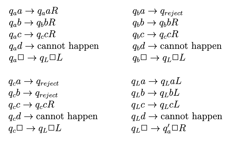
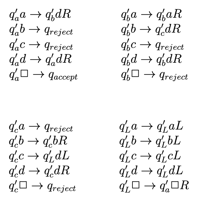
Transition function:
We now need to encode the logic for the above states into the transition funciton. Each rule will have the form \(q\sigma \rightarrow q'\sigma'M\), where \(q, q'\) are the input and output states, \(\sigma, \sigma'\) are the symbols read and written by the tape head, and \(M\) is a move instruction.
Here it is - cheat sheet copied from the book because I didn’t have time to put it in the tabular format I prefer for one-tape machines: